Supporting materials
Download
Download this article as a PDF


Three simple experiments illustrating Faraday’s law of induction and the different ways induced currents may be generated.
In this article, we present a series of simple classroom experiments that allow students to observe magnetic induction phenomena directly and apply their knowledge of induced currents to explain them.
When students are able to interact directly with the subject matter, they are more engaged, involved and motivated. This leads to a more gratifying and effective learning and teaching experience for students and teachers. As the old Chinese proverb goes, “I hear and I forget; I see and I remember; I do and I understand”.
The activities are aimed at students aged 16 to 19. We recommend that students carry out the experiments in groups of three and then discuss their results before presenting them to the whole class.
After completing this activity, students should
Back in 1831, the English scientist Michael Faraday discovered that it was possible to generate electricity by means of motion in a magnetic field. He also demonstrated how a current in one circuit could induce a current in a neighbouring circuit. He soon explained this phenomenon in terms of variation in magnetic flux. The following year, in 1832, the American scientist Joseph Henry made similar observations independently.
These findings eventually led to the formulation of Faraday’s law of induction, which is now one of the four fundamental laws of electromagnetism. This law states that the electromotive force Ɛ induced in a circuit is proportional to the rate of change of the magnetic flux through the circuit. Faraday’s law is expressed mathematically as follows:
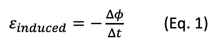
The minus sign on the right-hand side of the equation indicates that the direction of the induced current generates a field that opposes the change in the magnetic flux that caused the current in the first place (Lenz’s law).
There are different ways to change the magnetic flux through a circuit and, consequently, various ways in which a current can be induced. We will explore these in the proposed activities.
The magnetic flux (Ø ) through a given surface can be thought of as the number of magnetic field lines that pass through it.
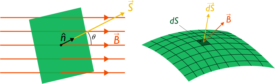
Consider a flat loop described by a surface vector, where the magnitude of this vector is equal to the loop’s surface area and the vector’s direction is perpendicular to the loop. In the presence of a uniform magnetic field, the flux through the loop is expressed as the scalar product ofand:
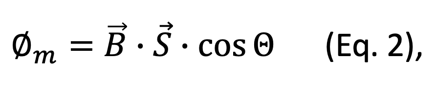
Where θ represents the angle betweenand(see figure 1a).
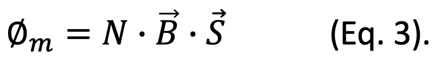
If we have a coil of N turns instead of a closed loop, the magnetic flux will increase N-fold, as the magnetic field penetrates each of the loops forming the coil:
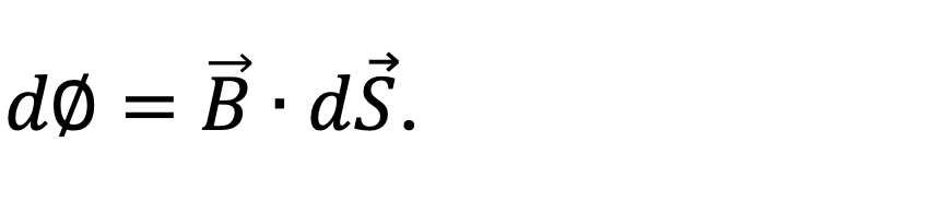
When the magnetic field is non-uniform and the surface through which the flux must be calculated is not flat, the surface can be divided into small parts represented by d. This so-called differential surface element, d, is small enough that we can consider that the magnetic field through it to be constant (see figure 1b). The flux differential dØ through d is therefore:
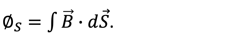
The flux through the entire surface is equal to the sum of all the flux differentials dØ through their respective differential surface elements and can be obtained by integrating:
Combining this equation with Faraday’s law, we can see that a current can be induced in a closed loop in any of the following ways:
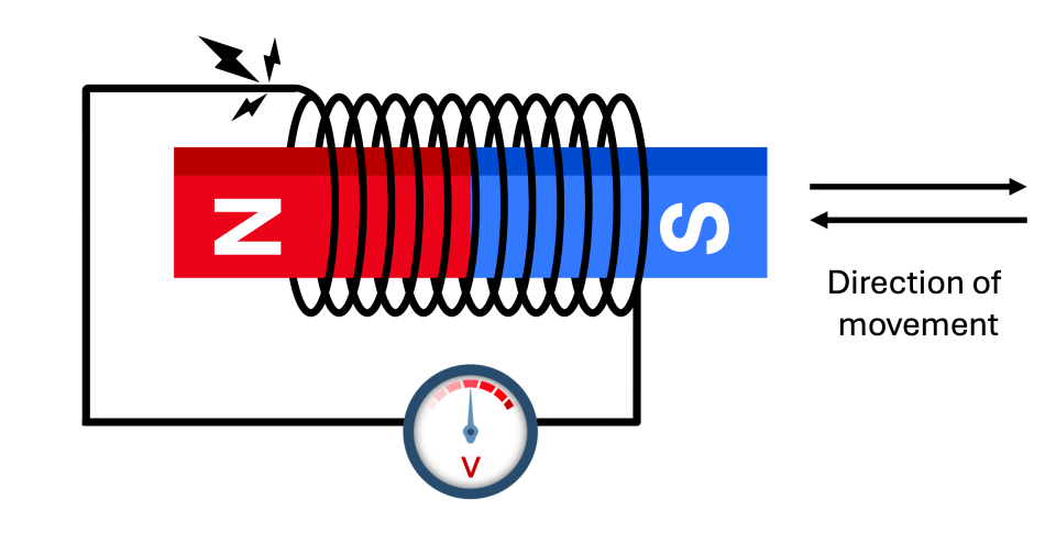
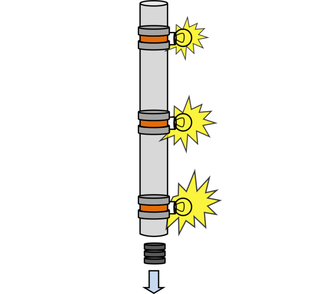
In this activity we will induce an electrical current by changing the magnitude of the external magnetic field.[1,2]
Observation: As the magnet falls through the tube with the three coils, the light bulbs are observed to flash one after the other. The intensity of each successive flash increases.
Explanation: Due to the uniform accelerated motion of the falling magnet, its velocity – and therefore the change in flux through each successive coil – increases as it falls.[3]
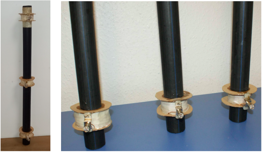
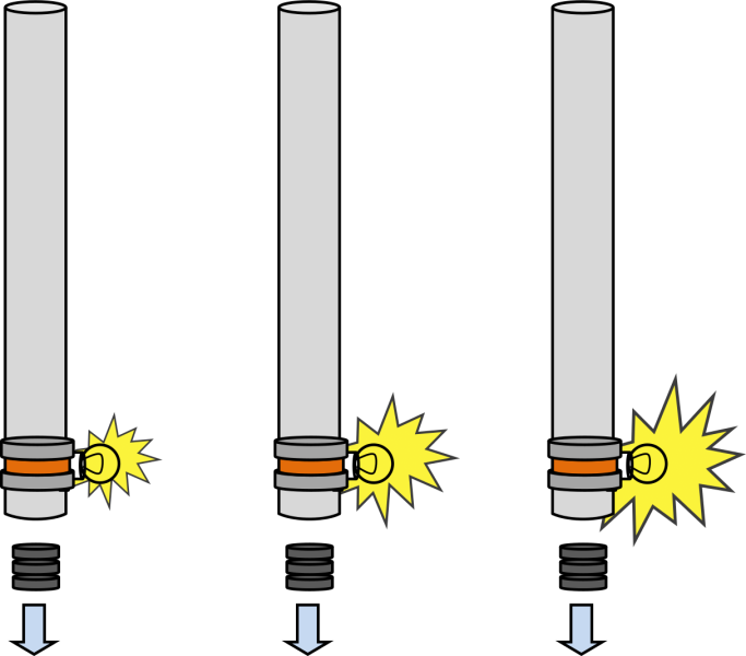
Observation: The falling magnets produce flashes of different intensity in each of the three tubes. The greater the number of turns, the more intense the flash.
Explanation: The magnetic flux, and therefore the induced current and the intensity of the flash, is proportional to the number of turns in the coil.
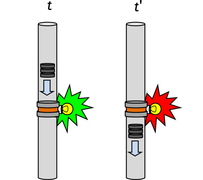
Observation: When the magnet is dropped through the tube, the red and green LEDs flash quickly in succession, not simultaneously. When the orientation of the magnet is reversed, the order of the flashes changes (red-green vs green-red).
Explanation: The change in flux is positive (i.e., flux increases) when the magnet approaches the coil, and negative (i.e., flux decreases) when it moves away from it. Therefore, the induced current first flows in one direction, allowing only one of the LEDs to flash, and then in the other direction, causing the other LED to flash (see figure 5). (The two LEDs are connected in opposite orientations).
The following questions can help you evaluate how well the students have grasped the concepts:
A detailed discussion of the experiments can be found in the explanation sheet 1 in the supplementary materials.
In this experiment we will induce a current by changing the surface area of a coil immersed in a magnetic field.[4]
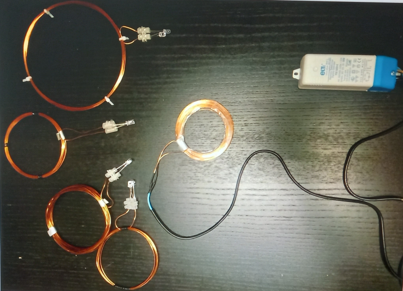
We used the following materials to build the set-up shown in figure 6.
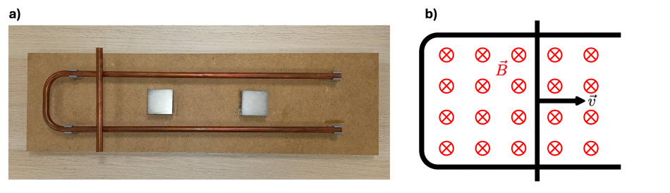
Assemble the materials as shown in figure 6a.
Observation: As the rod rolls over the rails, it appears to be slowed down.
Explanation: As the rod rolls to the right, the flux through the closed circuit formed by the rods increases, inducing an EMF. A current now flows through the moving rod. Being immersed in the magnetic field produced by the magnets, the current is subject to a magnetic force that opposes its motion.
The following questions can help you evaluate how well the students have grasped the concepts:
A detailed discussion of the experiments can be found in the explanation sheet 2 in the supplementary materials.
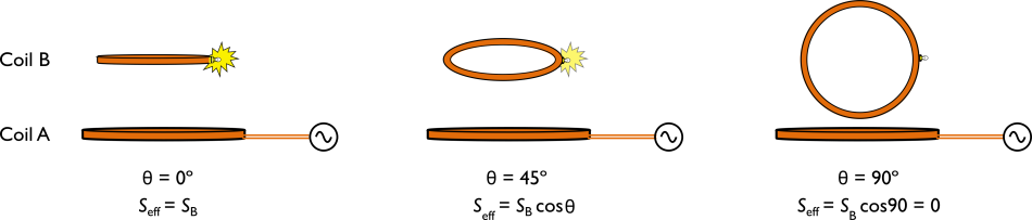
In this last activity we will explore the effect of the relative orientation of the coil and the magnetic field on the induced current.[4]
Observation: When coil B is placed above coil A, the LED lights up. When coil B is parallel to coil A (θ = 0°), the LED intensity is highest. As coil B is rotated with respect to coil A, the intensity decreases continuously until it disappears completely when coil B is perpendicular to coil A (θ = 90°).
Explanation: The alternating current (AC) in coil A produces a flux variation in coil B, which induces an AC current in coil B. As coil B rotates, the flux through it decreases until it reaches 0 when the coils are perpendicular.
The following questions can help you evaluate how well the students have grasped the concepts:
A detailed discussion of the experiments can be found in the explanation sheet 3 in the supplementary materials.
The activities proposed in this article will help students develop an intuition with regards to Faraday’s law of induction and Lenz’s law by means of three hands-on experiments exploring the concept of magnetic flux. The three different experimental set-ups allow students understand the dependence of the magnetic flux on the magnetic field, the circuit’s surface area and the relative orientation of the two.
[1] Del Mazo A (2002) Experiencias en electromagnetismo. Didáctica de las Ciencias Experimentales 34: 94–103.
[2] Anta A, Sancho C (2011) Experimentos e investigación en física. In Caamaño A (eds) Física y Química: Investigación, innovación y buenas prácticas pp 105–129. Graó. ISBN: 978-84-9980-081-3
[3] Amrani D (2005) Electromotive force: Faraday’s law of induction gets free-falling magnet treatment. Physics Education 40: 313–314. doi: 10.1088/0031-9120/40/4/F02
[4] Tipler PA ; Mosca G (2010): Ley de Lenz. In Casas-Vázquez J (eds) Fisica: Para La Ciencia Y La Tecnologia pp 965-972. Editorial Reverté. ISBN: 978-84-291-4430-7
Download this article as a PDF
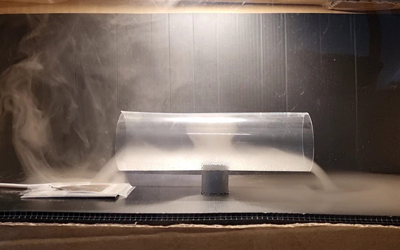
Do air convection currents really move as they are drawn in textbook illustrations? Let’s make invisible convection currents visible using mist.


Explore the science of sound and electromagnetism with this practical build-it-yourself…


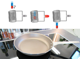
Explore electromagnetic induction and of one of its well-known applications – the induction hob – with these hands-on…