Supporting materials
Download
Download this article as a PDF


Small but mighty: investigate the role of herbaceous plants in the school garden for their contribution to biodiversity and sequestering carbon dioxide.
Carbon dioxide (CO2) constitutes about 0.04% of the atmosphere and is a greenhouse gas. CO2 emissions have increased since the Second Industrial Revolution, contributing to anthropogenic global warming.
Trees play an important role in sequestering CO2, and it has been calculated how many trees are needed to support human activities,[1] but what about the role of herbaceous plants that grow spontaneously in courtyards or lawns in sequestering CO2 or in contributing to biodiversity? By applying knowledge of biology and chemistry, through an inquiry-based learning (IBL) approach, it is possible to convey complex concepts[2] and achieve the following goals:
Learning objectives
Cultural objectives
The project is aimed at students aged 15–17. Ideally, they should already be familiar with taxonomic ranks; biomolecules and their chemical composition; the carbon cycle and photosynthesis; and moles, molar mass, and molar volume under standard ambient temperature and pressure (SATP).
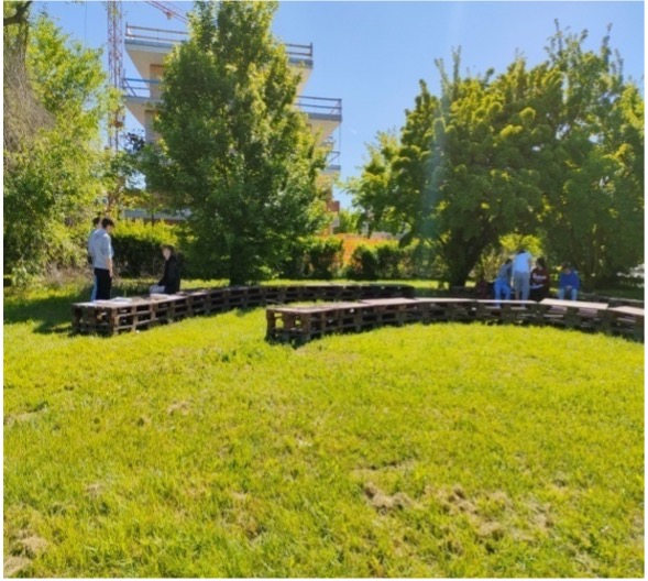
The aim of this activity is to investigate the biodiversity of herbaceous species in a lawn or meadow, for example, in the school garden.
Students use an app to identify herbaceous species and determine their frequency in the sampled areas. They then create a digital herbarium and assign their own biodiversity index to compare the areas.
This activity is suitable for students aged 15–17 and takes approximately six lessons to complete.
Location notes
If the school lacks a garden or park, or if the existing one is too small to accommodate the biodiversity and biomass project, activities can be carried out with permission in a grassy area in a public or private park. Alternatively, a field that was once cultivated but has since been left to lie fallow could be used. The key is that the plants present should not have been intentionally sown but should be the result of spontaneous herbaceous growth, and human intervention should be limited to occasional mowing. If no areas with these characteristics can be found, then areas with more significant human intervention can be used. However, it is essential to highlight this aspect for students. This will enable a discussion on the impact of human activities on biodiversity and the importance of preserving natural areas.
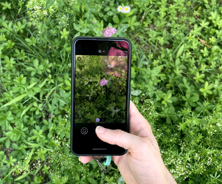
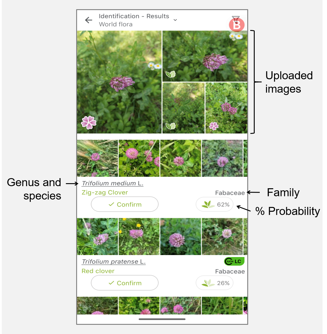
Pl@ntNet is a citizen-science project for plant identification based on machine learning, and is available as an app. The Pl@ntNet app is a convenient tool to identify herbaceous species, but it is important to consider its reliability.[3–6]
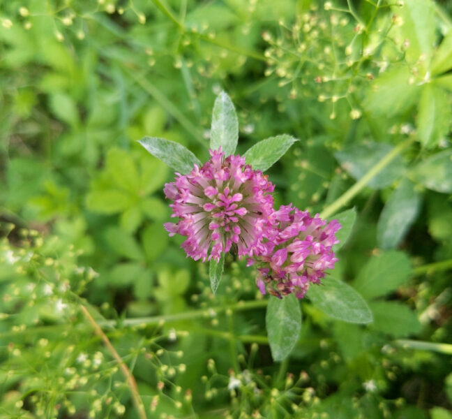
It is important to analyze intact plants, preferably providing several photos showing different structures like leaves and flowers, otherwise the reliability of the Pl@ntNet application decreases. It is important to take good images that are well-framed and sharply focused. Results with probability of identification less than 60% are excluded.
Not only Pl@ntNet but also other apps like iNaturalist can be used to identify species.[7]
Note: printable data tables are provided but processing the data will be much easier if spreadsheets are used after the initial data recording.


An example dataset is shown in the supporting material. Below are the processing results.
| Sample area no. | Biodiversity index |
|---|---|
| 1 | 7-11 |
| 2 | 7-11 |
| 3 | 10-17 |
| 4 | 6-09 |
| 5 | 7-14 |
| 6 | 6-09 |
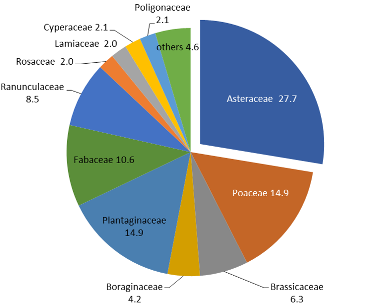
| Family | No. of genera (list them) | No. of species |
|---|---|---|
| Asteraceae (or Compositae) | 7 (Bellis, Crepis, Hypochaeris, Lactuca, Leontodon, Sonchus, Taraxacum) | 13 |
| Poaceae | 6 (Agrostis, Brachipodium; Eragrostis, Lolium, Phleum, Poa) | 7 |
| Brassicaceae | 3 (Arabidopsis, Cardamine, Capsella) | 3 |
| Plantaginaceae | 2 (Plantago, Veronica) | 7 |
| Fabaceae | 2 (Medicago, Trifolium) | 5 |
| Boraginaceae | 2 (Myosotis, Symphitum) | 2 |
| Ranunculaceae | 1 (Ranunculus) | 4 |
| Lamiaceae | 1 (Lamium) | 1 |
| Rosaceae | 1 (Potentilla) | 1 |
| Cariophyllaceae | 1 (Cerastium) | 1 |
| Cyperaceae | 1 (Carex) | 1 |
| Marsileaceae | 1 (Marsilea) | 1 |
| Polygonaceae | 1 (Rumex) | 1 |
| Total | 29 genera | 47 species |
Below are examples of questions to consider by looking at the data:
For example, after analyzing and discussing the example data shown above, students concluded the following:
Sample area No. 3 has greatest biodiversity (Data table 3). The presence of different species in the sample areas shows that the garden is not homogeneous, and thus, confirms the spontaneous origin of the plants. Sporadic cutting and low maintenance allow the establishment of many herbaceous species, generally considered weeds, which are carriers of great biological diversity.
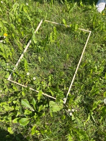
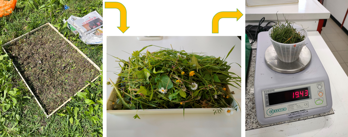
The purpose of this activity is to investigate the biomass of a lawn. Students calculate how much CO2 has been removed from the atmosphere to constitute the organic above-ground part of the grass/plants present in 1 m2 of lawn or garden by applying a mole quantity calculation.
This can be carried out in any area that hasn’t been mowed recently. For practical reasons, if the quantity of plant material taken from the rectangular sample is large, it will not all be dehydrated. Three small portions are easier to handle and dehydrate.
This activity is suitable for students aged 15–17 and takes five lessons to complete.

Below are examples of the data collected and results of its processing. The activity was carried out on three different dates, from April to May, by three different classes of students.
| Sampling date | Water (% m/m) | Dry biomass (g/m2) | CO2 (g/m2) | CO2 (l/m2) |
|---|---|---|---|---|
| 10 April | 77.18 | 86.91 | 146.58 | 82.58 |
| 18 April | 77.23 | 127.51 | 15.06 | 121.22 |
| 4 May | 78.36 | 257.96 | 435.10 | 245.13 |
Students calculate the number of moles of carbon in the biomass then, knowing that one mole of carbon comes from one mole of CO2 through photosynthesis, they determine the grams and litres of CO2 that have been removed from the atmosphere. The teacher collects the Excel worksheets, checks the procedure and the results obtained, and discusses with the class if there are errors.
Note that the calculations underestimate the absorbed CO2 because only the aerial parts of the plants are used and we don’t consider the root biomass. The data demonstrates the importance of herbaceous plants, which, growing spontaneously in uncultivated land, trap CO2 very effectively, thanks to their fast growth.[12]
The results only provide information about the sampling instant. Subsequent studies could aim to find the correlation between the amount of CO2 that is converted into biomass over a time interval (e.g., a month or a season) in association with factors like the average temperature, relative humidity, precipitation, and light intensity on the school lawn.
Thanks to the students of the 2nd C and 2nd M classes at the scientific high school “Liceo Statale Galileo Galilei” (Dolo, Venice), who worked hard and were the first to experiment with Activities 1 and 2 in the 2022–23 school year. I also thank my former colleague, high school teacher Elisa Cappelletto, who initially collaborated on the realization of the project with the 2nd F class.
[1] Schwarz A et al. (2024) How much carbon is locked in that tree? Science in School 67: 1–7.
[2] Wahyuni L et al. (2022) The effect of guided inquiry learning model through the utilization of school environment towards students’ scientific literacy on biodiversity concepts. International Journal of Biology Education towards Sustainable Development 2: 44–52. doi: 10.53889/ijbetsd.v2i1.131
[3] Affouard A et al. (2021) Customized e-floras: how to develop your own project on the Pl@ntNet platform. Biodiversity Information Science and Standards 5: e73857. doi: 10.3897/biss.5.73857
[4] Pl@ntNet: an app to advance botany: https://www.cirad.fr/en/our-activities-our-impact/our-impact/success-stories/pl-ntnet
[5] Affouard A et al. (2023) Pl@ntNet observations. Pl@ntNet. Occurrence Dataset. doi: 10.15468/gtebaa
[6] Joly A et al. (2016) A look inside the Pl@ntNet experience. Multimedia Systems 22: 751–766. doi: 10.1007/s00530-015-0462-9
[7] Echeverria A et al. (2021) Learning plant biodiversity in nature: the use of the citizen–science platform iNaturalist as a collaborative tool in secondary education. Sustainability 13: 735. doi: 10.3390/su13020735
[8] GBIF: Global Biodiversity Information Facility: https://www.gbif.org/
[9] Index of botanical species present in Italy: https://www.actaplantarum.org/flora/flora.php?m=0
[10] Ma S et al. (2018) Variations and determinants of carbon content in plants: a global synthesis. Biogeosciences 15: 693–702. doi: 10.5194/bg-15-693-2018
[11] The types and characteristics of biomass (table on p 18): http://bioenergy-fvg.uniud.it/fileadmin/documenti/Corso_energie_rinnovabili/Le_tipologie_e_le_caratteristiche_delle_biomasse.pdf
[12] Di Vita et al. (2017) A review of the role of vegetal ecosystems in CO₂ capture. Sustainability 9: 1840. doi: 10.3390/su9101840
European Molecular Biology Laboratory (EMBL)
The European Bioinformatics Institute (EMBL-EBI) has launched the Global Biodiversity Portal, an open-access platform that brings together genomic data from different biodiversity projects within the Earth BioGenome Project. The portal enables global biodiversity research by providing centralized, accessible data for understanding the genetic uniqueness and adaptability of species and supports practical applications, such as agriculture and bioengineering. The portal simplifies access to genome sequence data and allows users to easily search for species information.
Download this article as a PDF
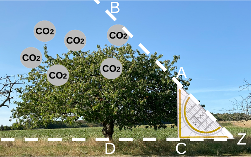
Biology, maths, and the SDGs: estimate the CO2 absorbed by a tree in the schoolyard and compare it to the CO2 emissions of a short-haul flight.

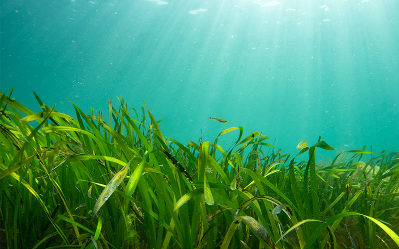
Did you know that there are flowering plants that live in the sea? The unique characteristics of seagrasses are vital for the health of our planet.


A walk on the wild side: invite some ants to take a walk on your petri dish and discover how bacteria from their feet could help us reduce pesticide use.