


Galileo and the moons of Jupiter: exploring the night sky of 1610 Teach article
Learn how you and your students can use mathematics to study Jupiter’s moons.

(Justus Sutermans, 1636)
Public domain image; image
source: Wikimedia Commons
On a January night in 1610, Galileo Galilei looked at Jupiter through his telescope and saw what he thought were three stars near the planet. He continued his observations for about two months, and over this time realised that there were actually four ‘stars’, which changed their position around Jupiter. Galileo concluded that the ‘stars’ were in fact planets orbiting Jupiter – the Medicean planets, as he named them at the time, but which are now known as the Galilean moons in honour of their discoverer (figure 1).
‘… I should disclose and publish to the world the occasion of discovering and observing four PLANETS, never seen from the very beginning of the world up to our own times….”
Galileo Galilei in Sidereus Nuncius (Starry Messenger; 1610)

Galilean moons Io, Europa,
Ganymede, and Callisto
(Jupiter is not on the
same scale as the satellites).
Image courtesy of NASA
Planetary Photojournal
This discovery of Galileo’s forms the basis of a project that I devised for my 12th-grade physics students (17–18 years old) when teaching the topic of simple harmonic motion. The project builds on a similar activity I developed earlier, about the motion of the Galilean moon Io (Ribeiro, 2012). The current project is enquiry-based, and aims to engage students with a rich variety of scientific processes – from exploring historical contexts to obtaining and analysing experimental results and communicating their conclusions to others.
The aim of the project is for your students to prove that Galileo was right when he claimed that the ‘stars’ near Jupiter were in fact the planet’s satellites. To do this, students collect data about the movement of the moons using a computer simulation, and then show that this movement has the characteristics of simple harmonic motion, with Jupiter as the centre. At the end of the project, students produce a report (a document or presentation) to describe their findings and the whole process – and, ideally, share this with students from other countries so they can learn to communicate scientific work internationally.
The duration of the project will vary depending on how the teacher decides to approach it. I spent four months working on the project with my students, but if you do not have time to run the whole project with your students, you could select individual activities from it.
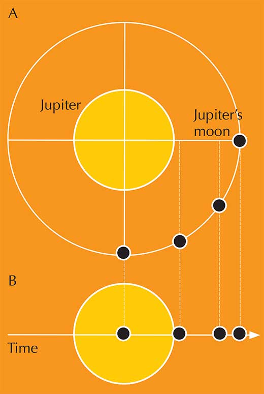
one of the Galilean moons
around Jupiter: A) as seen
from above the orbit plane
and B) as seen from Earth
(viewed parallel to the orbit
plane). The black dots
represent the Galilean
moon’s positions at equal
intervals of time. Click on
image to enlarge.
Image courtesy of Carla Isabel
Ribeiro
Simple harmonic motion and uniform circular motion

Image courtesy of Nicola Graf
Simple harmonic motion (SHM) is the term used to describe regular periodic motions such as the swinging of a pendulum or the oscillations of an object attached to a spring. Plotting a graph of these motions (distance from the central point against time) produces the characteristic form of a sine wave (figure 2).
SHM can be interpreted as a projection onto one axis of an object that is moving with a uniform circular motion (UCM). For example, imagine an object moving in a circle in a horizontal plane. If we view this from the side at ‘eye level’ (equivalent to projection onto the x axis), we see a to-and-fro motion exactly the same as that of an oscillating object attached to a spring. Only when viewing the motion from above would we see the movement as circular.
This relationship between SHM and UCM can be applied to the Galilean moons as seen from Earth: their movement appears to be SHM, due to the projection of their UCM around the planet onto our direction of vision (figure 3). (The orbits are slightly eccentric, but only to a small degree, so the moons can be considered to have a circular orbit and to move at constant speed.)
Cosmology in Galileo’s time
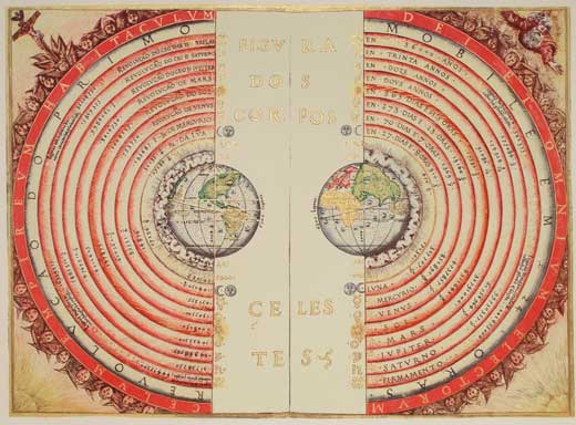
geocentric model of the
cosmos, depicted in
Bartolomeu Velho’s
Cosmographia (1568).
Click on image to enlarge.
Public domain image; image
source: Wikimedia Commons
Galileo’s observations of Jupiter’s moons were made during a time of scientific transition, from the geocentric (Earth-centred; figure 4) model of Aristotle and the Catholic Church to the heliocentric (Sun-centred) model.
Galileo, of course, was to take up the heliocentric model explicitly some years later, in a direct challenge to Catholic doctrine. However, his telescopic observations, published in his book Sidereus Nuncius (Starry Messenger) in 1610, were already causing friction by contradicting the teachings of Aristotle. In Aristotle’s model, everything in the cosmos orbits Earth – so the idea of moons orbiting the planet Jupiter was at odds with this.
The project step by step
Step 1: 17th century cosmology
Ask your students to research the cosmological ideas that were current in early 17th century Europe. What effect might they have had on Galileo, his investigations and conclusions? Students should also read excerpts from Starry Messengerw1, in which Galileo describes his observations and conclusions.
Step 2: choose the planetarium software
You will need to download the freeware planetarium programme Stellariumw2 or a similar simulation. Then divide your students into four groups, and assign each group to one of the four Galilean moons (Io, Callisto, Ganymede or Europa).
Step 3: tracking Jupiter’s moons
Ask your students to use Stellarium to investigate the position of their moon over time: in a table, each group should record the displacement (x) – the distance of their moon from the centre of Jupiter – at a succession of times (t). They will also need to find the maximum displacement (A) of the moon from the planet’s centre.
Measurements should be taken at intervals that differ between the four moons, depending on their distance to the planet and, therefore, their orbital period. The students should use trial and error to find the most appropriate interval for their moon. Their aim is to obtain at least 10 measurements, one of which should be A.
For example, Io is the moon that is closest to Jupiter, which means it orbits most quickly. If the students take their measurements at 1 h intervals, the data will not be sufficient; 15 min intervals would be more appropriate. For one of the more distant Galilean moons, 15 min intervals would result in more data than is necessary, so a longer interval should be used.
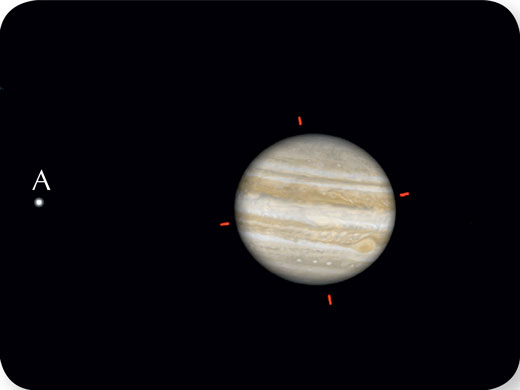
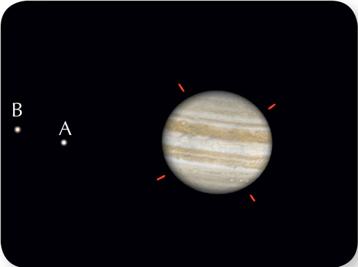
To find the centre of the planet on Stellarium, your students can use the red marks around Jupiter (figure 5) to draw two lines that cross at its centre. To find the distance from that point to the moon being studied, they can either use an image programme or print off the screenshots and measure the distances with a ruler.

freeware programme
Stellarium of Jupiter and its
moons Europa (A) and Io (B).
Click on images to enlarge.
Images courtesy of Stellarium
Step 4: testing Galileo’s conclusion
The fourth and most complicated step is for students to show that Galileo was right when he concluded that the SHM he observed is produced by a moon’s UCM around its planet.
To find the orbital period T of their moon, the students will need the mathematical equation for SHM:
x = A × sin(ω t + φ) (1)
where w is the angular frequency and j is a constant (the phase constant), together with the equation linking w and T:
ω = 2π / T
where x is the displacement, A the amplitude of the motion or maximum displacement, t is the time and φ is a constant (the phase constant).
Equation (1) can be transformed into the linear equation (2), thus:
x = A × sin(ω t + φ) (1)
→ x / A = sin(ω t + φ)
→ arcsin(x / A) = ω t + φ
Since ω = 2π / T
→ arcsin(x / A) = (2π/ T)t + φ (2)
If your students observe an object behaving according to equation (2) – which describes SHM – then it is reasonable to conclude that it is orbiting the planet as a moon.
Because equation (2) is linear, we can see that if your students use their data from step 3 to plot a graph of arcsin(x / A) against t, the gradient will be 2π / T, from which they can easily calculate the orbital period T. The phase constant of the moon, φ, is the intercept on the y axis. Figure 6 shows an example of a graph that your students could plot using data for the moon Europa.

Image courtesy of Carla Isabel Ribeiro
The graph above has a gradient of 0.0741.
Since the gradient is equal to 2π/ T, it follows that:
2π / T = 0.0741
→ T = 2π / 0.0741
= 84.8 h
The more mathematically able students could then carry out a regression analysis of the data to test the ‘goodness of fit’ to equation (2). The value obtained in the case of Europa (R2 = 0.998) shows that the data comply closely with the equation, and thus confirms that this object behaves like a moon in orbit.
The accepted value for Europa is about 3.55 days (85.2 h), which is quite similar to the value calculated above. The difference between the two values can be a good starting point for a discussion about the accuracy of experimental results. What might have gone wrong? Were any errors random or systematic?
In this case, the error may have its origin in the measurement of A, since the moon’s positions were simulated 1 h apart, and the maximum displacement could have been reached between two measurements. You could ask your students to suggest ways to minimise this error.

Doge of Venice how to use
his telescope (HJ Detouche,
1754). Click on image to
enlarge.
Public domain image; image
source: Wikimedia Commons
Step 5: presenting the results
The last step is for each group of students to present their work, describing the whole investigation and showing their results. In science, it is important to communicate, so you could get your students to make their presentations to students in another class, or perhaps as part of a school fair or open day. They should think about how best to communicate their work. How can they make it simple for others to understand? What images could they use to help explain what they did?
More ambitiously, you could even set up a collaboration with a school in another country. Scientists sometimes have to communicate in foreign languages – often, but not always, English. Based on this project, I am hoping to set up an international collaboration through the eTwinning networkw3. On a smaller scale, I would also be happy to hear from other schools that would like to work together on the project.
References
- Ribeiro CI (2012) Io and its simple harmonic motion. Physics Education 47: 268-270. doi: 10.1088/0031-9120/47/3/F04
Web References
- w1 – Download a recent English translation of Sidereus Nuncius (Starry Messenger), Galileo’s famous early work describing discoveries made with the telescope. Pages 17 and 18 contain his observations of the moons of Jupiter for the dates featured in this project.
- The original edition is also available online.
- w2 – Stellarium, the planetarium simulation used in the project, can be downloaded free of charge.
- w3 – The eTwinning website promotes school collaboration in Europe through the use of information and communication technologies (ICT). Available in 23 languages, it has nearly 50 000 members and more than 4000 registered projects between two or more schools across Europe.
Resources
- The Physclips website offers a clear explanation of simple harmonic motion, with video and animation.
- NASA’s Solar System Exploration website offers up-to-date information about Jupiter and its moons, including space missions.
- For an article describing a similar project exploring the Galilean moons, using a telescope equipped with a charge-coupled device (CCD) camera, see:
- de Moraes IG, Pereira JAM (2009) Using simple harmonic motion to follow the Galilean moons – testing Kepler’s third law on a small system. Physics Education 44: 241. doi: 10.1088/0031-9120/44/3/002
- The article can be downloaded free of charge from the website of the University of Picardie, France.
- Project CLEA (Contemporary Laboratory Experiences in Astronomy), hosted by Gettysburg College, USA, offers laboratory exercises that illustrate modern astronomical techniques. Each exercise consists of a dedicated computer programme, a student manual, and a technical guide for the teacher. Several of the exercises involve Jupiter’s moons.
Review
This article suggests a new enquiry-based way of teaching simple harmonic motion: students use their knowledge of mathematics, physics and information and communication technology to characterise the motion of Jupiter’s moons. They collect data from a software programme, process it and then plot graphs, particularly of sine and arcsine functions, to calculate the moons’ orbital periods.
The interdisciplinary nature of the article serves to make science more enjoyable. In addition, the activity develops soft skills such as the presentation of results and communication. By joining an international project, the students would have the opportunity to share their results not only with other members of their class but with students from different countries.
Corina Toma, Computer Science High School “Tiberiu Popoviciu” Cluj Napoca, Romania